Hello everyone,
I will share a project for with you about deep learning and neural network. Actually, i improved last year this project. But i forgot shared. With this project you can decomposition cats and dogs photos. I used pyhton language this project. You can see project files down below.
If you want, firstly i can describe this project.
FIRST STEP : IMPORT LIBRARIES
import osimport cv2import numpy as npfrom skimage.io import imreadfrom skimage.transform import resizeimport matplotlib.pyplot as pltfrom tensorflow.keras import layersfrom tensorflow.keras.optimizers import Adamfrom tensorflow.keras.applications import VGG16from tensorflow.keras.models import Model, Sequentialfrom mlxtend.plotting import plot_confusion_matrixfrom sklearn.model_selection import train_test_splitfrom sklearn.metrics import roc_curve, auc, confusion_matrix, classification_report,accuracy_scoreSECOND STEP : READ THE IMAGES AND RESIZE 150X150
def takeLabel(string):ifstring == "cats":return0else:return1images = []target = []base_dir = "dataset/"listdir = os.listdir(base_dir)for sub_dir in listdir:label = takeLabel(sub_dir)sub_dir = os.path.join(base_dir,sub_dir)list_sub_dir = os.listdir(sub_dir)forfileinlist_sub_dir:file_path = os.path.join(sub_dir,file)try:img = imread(file_path)img = cv2.cvtColor(img, cv2.COLOR_BGR2RGB)dimension=(150, 150)img_resized = resize(img, dimension, anti_aliasing=True, mode='reflect')images.append(img_resized)target.append(label)except:print(file_path)THIRD STEP : CONVERT DATA INTO NUMPY ARRAY
x_data = np.array(images)y_data = np.array(target)FOURTH STEP : PLOT SAMPLE PICTURE
Firstly cat;
plt.imshow(images[85])
Secondary, dog;
plt.imshow(images[1680])
FIFTH STEP : SPLIT DATA INTO TRAIN, VALIDATION AND TESTING
x_train,x_test_val,y_train,y_test_val = train_test_split(x_data,y_data,test_size=0.4,random_state=45)x_val,x_test,y_val,y_test = train_test_split(x_test_val,y_test_val,test_size=0.4,random_state=45)SIXTH STEP : MODEL ARCHITECTURE OF VGG16
vgg_16 = VGG16(weights='imagenet',include_top=False,input_shape=(150, 150, 3))vgg_16.summary()…
model = Sequential()model.add(vgg_16)model.add(layers.Flatten())model.add(layers.Dropout(0.5))model.add(layers.Dense(1, activation='sigmoid'))model.layers[0].trainable = Falsemodel.compile(loss='binary_crossentropy',optimizer=Adam(learning_rate=1e-4),metrics=['acc'])model.summary()SEVENTH STEP : FITTING THE MODEL
history = model.fit(x_train,y_train,validation_data=(x_val,y_val),epochs=100,batch_size=32)…
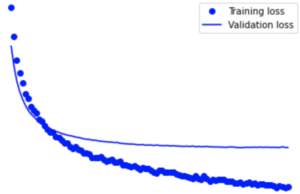
EIGHTH STEP : PLOT GRAPH OF ACCURACY AND LOSS DURING TRAINING
%matplotlib inlineacc = history.history['acc']val_acc = history.history['val_acc']loss = history.history['loss']val_loss = history.history['val_loss']epochs = range(1, len(acc) + 1)plt.plot(epochs, acc, 'bo', label='Training acc')plt.plot(epochs, val_acc, 'b', label='Validation acc')plt.title('Training and validation accuracy')plt.legend()plt.figure()plt.plot(epochs, loss, 'bo', label='Training loss')plt.plot(epochs, val_loss, 'b', label='Validation loss')plt.title('Training and validation loss')plt.legend()plt.show()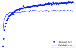
AND PREDIC THE RESULT
y_pred=model.predict(x_test)y_predicted=[]for i in y_pred:ifi>=0.5:y_predicted.append(1)else:y_predicted.append(0)ACCURACY SCORE
print('Accuracy of the model on testing dataset %0.2f %%' % (accuracy_score(y_predicted,y_test)*100))CONFUSION MATRIX
CR=confusion_matrix(y_test, y_predicted)fig, ax = plot_confusion_matrix(conf_mat=CR,figsize=(10, 10),show_absolute=False,show_normed=True,colorbar=True)plt.show()
SENSITIVITY AND SPECIFICITY
print(classification_report(y_test, y_predicted))ROC CURVE
fpr, tpr, thresholds = roc_curve(y_test, y_predicted)roc_auc = auc(fpr, tpr)plt.figure()plt.plot(fpr, tpr, color='darkorange', lw=1, label='ROC curve (area = %0.2f)' % roc_auc)plt.plot([0, 1], [0, 1], 'k--', lw=1.5)plt.xlim([-0.05, 1.0])plt.ylim([0.0, 1.05])plt.xlabel('False Positive Rate')plt.ylabel('True Positive Rate')plt.title("ROC curve")plt.legend(loc="lower right")plt.show()
You can download this project is here…